Learning to defer in practice: A retrospective example with real chest X-rays and human annotations

What this example demonstrates

Imagine a model reviewing a chest X-ray for several possible findings. It can answer every question itself, or it can pass selected decisions to a radiologist. The useful system is not necessarily the one that automates the most. It is the one that gives each decision to whoever is more likely to get it right.

This retrospective experiment uses real chest X-rays and real human annotations to make that idea concrete. I compare a familiar baseline— send the model's least confident findings to a radiologist—with one-vs-all learning to defer (OvA-L2D), and include random deferral as a sanity check. OvA learns something more useful than uncertainty alone: how likely the model and the available expert are to be correct on each decision.

The data, briefly

I use 6,125 chest X-rays from the radiologist-annotated VinDr-CXR dataset. Reader R9 is treated as the expert to whom the model can defer. The two other readers define the experimental reference: a finding is positive only when both mark it present, and a tie counts as absent. R9 never contributes to the reference used to judge R9.

I retain 17 findings with sufficient training support and split the data into 3,701 training, 1,209 validation, and 1,215 test images. A deferral applies to one finding on one X-ray—not necessarily the entire image.

The model

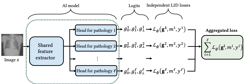
Both methods start from the same randomly initialised ResNet-18. Its image representation passes through a shared 256-unit layer, followed by one head per finding. The confidence baseline emits one binary logit per finding. OvA emits three: absent, present, and defer. The encoder and every head are trained end to end.

The multi-label architecture below shows that structure explicitly. The X-ray is encoded once, then each pathology head makes its own three-way OvA-L2D assessment. Each head receives an independent deferral loss, and those per-finding losses are summed to train the full model.

class L2DModel(nn.Module):
    def __init__(self, n_findings=17):
        super().__init__()
        # Keep the image features; discard ResNet's original classifier.
        self.encoder = resnet18(weights=None)
        self.encoder.fc = nn.Identity()

        # Compress the shared representation before branching by finding.
        self.shared = nn.Sequential(
            nn.Linear(512, 256), nn.ReLU(),
            nn.Dropout(0.1), nn.LayerNorm(256)
        )

        # Each head emits: absent, present, and defer.
        self.heads = nn.ModuleList([
            nn.Linear(256, 3) for _ in range(n_findings)
        ])

    def forward(self, images):
        h = self.shared(self.encoder(images))
        # Output shape: [batch, findings, 3].
        return torch.stack([head(h) for head in self.heads], dim=1)

The three outputs are not a softmax over mutually exclusive actions. OvA treats them as independent binary questions, each transformed by a sigmoid. That distinction is what lets the defer output represent an estimate of expert correctness.

The one-vs-all deferral loss

Where OvA fits historically

OvA was not the first consistent surrogate proposed for learning to defer. That earlier milestone came from Mozannar and Sontag (2020). They introduced a cost-sensitive reduction with a generalised cross-entropy loss that jointly learns a classifier and a rejector from examples of an expert's decisions. Their construction is consistent: with enough data and a sufficiently rich model, minimising the surrogate recovers the decision rule that minimises the combined machine–expert system's risk.

Verma and Nalisnick's 2022 OvA paper addressed a different issue. They showed that the earlier softmax formulation is not calibrated with respect to expert correctness; its parameterisation can even turn the derived expert-correctness score into something greater than one. OvA replaces that coupled softmax with independent binary problems for each class and for whether the expert is correct. The resulting sigmoid outputs can be interpreted as calibrated probabilities, while the loss remains a consistent surrogate for multiclass learning to defer. The point of OvA was therefore not to introduce consistency for the first time, but to preserve it while making the model's class and expert confidence estimates probabilistically meaningful. For those reasons, the OvA loss is a personal favourite of mine.

I use the notation from Verma and Nalisnick's paper first. Let $\mathcal{Y}=\{1,\ldots,K\}$ be the class set, $y\in\mathcal{Y}$ the reference label, $m\in\mathcal{Y}$ the expert's answer, and $g_1(x),\ldots,g_K(x),g_\perp(x)$the class and defer logits. Their point-wise OvA surrogate is Equation (8):

Here $\phi$ can be any suitable binary surrogate. The notebook uses the logistic loss:

The first two terms form $K$ one-vs-all class problems. The final line forms one more binary problem for expert correctness. When $m=y$, it reduces to $\phi(g_\perp(x))$; otherwise it reduces to $\phi(-g_\perp(x))$. This is exactly why the defer output is trained against whether the expert was correct.

For each binary chest X-ray finding in this notebook, $\mathcal{Y}=\{0,1\}$. Equation (8) is therefore implemented as three binary-cross-entropy-with-logits terms:

The three targets can be read directly as:

In the notebook, the three binary cross-entropies are summed for each image–finding pair, averaged across the batch, and divided by $\ln 2$ so the loss is measured in bits. That final scaling does not change the minimiser. A numerically stable PyTorch version is:

def ova_loss(logits, y, expert):
    # Targets for the absent and present logits.
    class_targets = F.one_hot(y.long(), num_classes=2).float()

    # The defer logit learns when this expert is correct.
    expert_correct = (expert == y).float()

    class_loss = F.binary_cross_entropy_with_logits(
        logits[..., :2], class_targets, reduction="none"
    ).sum(-1)
    defer_loss = F.binary_cross_entropy_with_logits(
        logits[..., 2], expert_correct, reduction="none"
    )

    # Sum the three OvA terms and report the batch mean in bits.
    return (class_loss + defer_loss).mean() / math.log(2)

This loss comes from Verma and Nalisnick, “Calibrated Learning to Defer with One-vs-All Classifiers” (ICML 2022). Their key result is that the OvA construction can yield calibrated estimates of expert correctness and is a consistent surrogate for the multiclass learning-to-defer objective. The notebook follows their released loss implementation.

Three ways to decide when to ask a human

The paper defines the classifier and hard rejector directly from the logits:

With logistic loss, the independent sigmoid outputs estimate class probability and expert correctness:

To draw a full performance curve across many deferral budgets, the notebook uses the corresponding continuous advantage score:

In words: defer where estimated expert correctness most exceeds estimated machine correctness. The confidence baseline instead trains a standard binary classifier, fits one temperature per finding using only validation data, and defers the least confident predictions first:

The baseline can identify model uncertainty, but it never learns where R9 is likely to help. That is the conceptual difference this comparison is designed to isolate.

Random deferral uses that same calibrated classifier but chooses which individual finding decisions to hand to R9 uniformly at random. I average 200 independent random orderings (seed 1), sampled without replacement, so every point still defers exactly the requested number of decisions. The routing score uses no labels, confidence, or expert correctness: it is a deliberately uninformed baseline.

How deferral helps

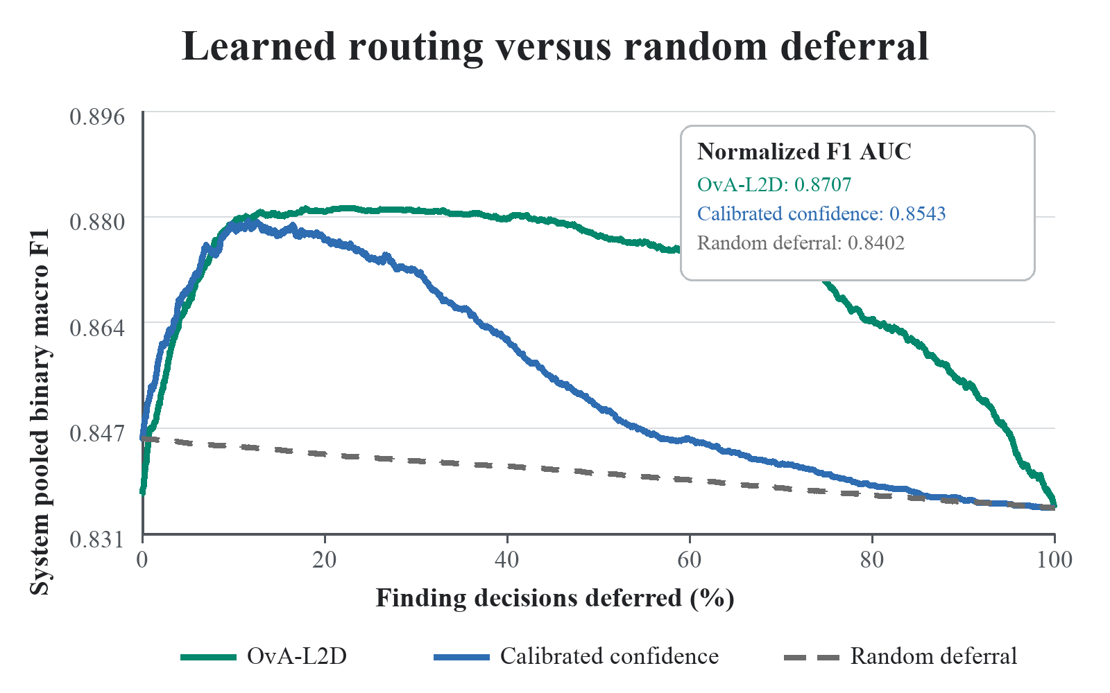
At 0%, each method uses machine predictions. Calibrated confidence and random deferral begin at exactly the same point because they use the same classifier. At 100%, every finding is sent to the same expert, so all three curves meet. Between those endpoints, random deferral shows what happens when the handovers contain no information about who is likely to be right.

Calibrated confidence improves on random routing while holding the machine fixed, which isolates the value of sending uncertain decisions first. OvA produces the best routing curve in this run because its ranking can also account for where the radiologist is likely to help—not merely where the model is unsure. The normalized F1 areas under the curve are 0.8707 for OvA-L2D, 0.8543 for calibrated confidence, and 0.8402 for random deferral.

That is the practical promise of learning to defer: a handover policy can improve the combined human–AI system without assuming that either participant is always better. It learns a division of work from their complementary patterns of success and failure.

Conclusion

Learning to defer is ultimately about allocating responsibility, not merely identifying uncertainty. This retrospective example suggests that modelling both machine and expert correctness can produce more useful handovers; the next step is to test such systems prospectively, with richer expert populations and coherent decisions across related findings.

References

- K. He, X. Zhang, S. Ren, and J. Sun. “Deep Residual Learning for Image Recognition.” Proceedings of CVPR, 2016. Paper
- H. Mozannar and D. Sontag. “Consistent Estimators for Learning to Defer to an Expert.” Proceedings of ICML, 2020. Paper
- R. Verma and E. Nalisnick. “Calibrated Learning to Defer with One-vs-All Classifiers.” Proceedings of ICML, 2022. Paper
- H. Q. Nguyen et al. “VinDr-CXR: An open dataset of chest X-rays with radiologist's annotations.” Scientific Data 9, 429, 2022. Paper
Limitations
This is a useful demonstration, not a prospective clinical evaluation. Several limitations matter when interpreting it:
- The experimental “ground truth” is agreement between only two clinicians, with ties counted as absent. It is an annotation reference, not an adjudicated diagnosis or patient-level clinical truth.
- Each of the 17 findings is deferred independently. Related findings can therefore be handed over in logically inconsistent ways—for example, predicting a specific child finding while deferring its implied parent. This is the problem we tackle in our NeurIPS paper; the CHL2D blog post explains why these incoherences arise and how we address them.
- R9 is a single, fixed expert observed during training. A deployed system would encounter clinicians with different expertise, workloads, and availability, including people it had never seen before.
- The analysis is retrospective. It does not measure how deferral would change a clinical workflow, turnaround time, radiologist behaviour, or patient outcomes.
- The learned models use one matched training seed, while the random baseline averages 200 routing permutations. Performance is summarised using pooled binary macro-F1. The area integrates F1 across deferral budgets; it is not ROC AUC, and it should not be read as evidence of statistical superiority.